Implementing a Virtual Machine in TeX that Runs Untyped Lambda Terms

This article introduces tex_of_ocaml¹, a half-joking OSS I developed. Readers are supposed to be somewhat familiar with untyped lambda calculi.

First appearance (written in Japanese):

• Dec 9, 2020. TeX言語で型なしλ計算を評価するVMを書いた話 - Qiita

Summary

tex_of_ocaml is publicly available at the following repository:

(the present article refers the implementation of commit hash e6e3997.)

This software consists of the following two components:

1. a small compiler implemented in Rust that transforms untyped lambda terms written in an OCaml-like syntax into TeX code, and
2. a back-end VM (i.e. bytecode interpreter) implemented in TeX that evaluates TeX code emitted by 1.

The former one is quite a simple compiler and does not do so notable performances². The most notable is the latter one; it implements Landin’s SECD Machine³ where produced TeX code is evaluated by full expansion (e.g. expansion by \edef).

In this way, an untyped lambda calculus can be embedded into a restricted version of TeX where only fully expandable operations are permitted, and this shows that TeX is Turing-complete even if it is restricted to fully expandable operations.

Example

You can try the software as follows:

Preparing input files

First, use the file in the repository:

examples/example3.txt

(fun x -> fun f -> f (arabic (add 1 x))) 42 (append "foo")

Here, add is the addition operation for natural numbers, arabic converts natural numbers to the string of their decimal representation, and append is the string concatenation.

Preparing an output environment

Create a directory _generated/ for outputs, and place secd.sty in it:

$ mkdir -p _generated
$ cp src_tex/secd.sty _generated

Compiling

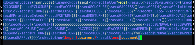
$ cargo run examples/example3.txt -o _generated/example3.tex

The generated file is like the following:

Executing the produced code

Run the produced code:

$ cd _generated
$ latexmk example3.tex

Then, a PDF file _generated/example3.pdf will be produced, and it looks like:

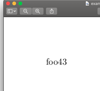
You can see that it says "foo43", the result of evaluating (fun x -> fun f -> f (arabic (add 1 x))) 42 (append "foo"). As a side note, integers and booleans can also be printed as a result on PDFs, in addition to strings⁴.

More elaborate computation, such as the one that calculates the factorial of an integer, can be run⁵:

examples/factorial.txt

let fix = (fun f -> (fun x -> f (fun v -> x x v)) (fun x -> f (fun v -> x x v))) in
let fact = fix (fun f -> fun n -> if iszero n then 1 else mult n (f (sub n 1))) in
fact 5

The compiler produces the following code,

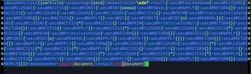
and it will result in the following PDF file as intended:

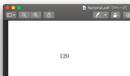
Hooray!

What is the full expansion?

Roughly speaking, the full expansion is a procedure of the TeX processor where only expansion (≒ term rewriting) is performed and imperative operations such as the assignment to registers are prohibited. As an example of situations where the full expansion is performed, executing \edef〈Command〉{〈Tokens〉} first fully expands 〈Tokens〉 and the resulting token list is used for defining how to rewrite 〈Command〉. During the full expansion, tokens that cannot be expanded are just skipped and appended to the resulting list when encountered⁶. This makes the full expansion a bit similar to the evaluation of purely functional languages.

Landin’s SECD machine

Although many papers or textbooks refer it, this section will briefly introduce Landin’s SECD Machine³. It is one of the ways to implement a virtual stack machine that emulates the evaluation of programs in a lambda calculus or some language like that. As the name suggests, it is formalized as a rewriting rules on quadruples consisting of \(S\) (Stack), \(E\) (Environment), \(C\) (Code), and \(D\) (Dump). These metavariables are defined by:

where \([X]^{\ast}\) ranges over (possibly empty) finite sequences of \(X\), and \(c\) ranges over the set of constants such as integers and Boolean values. The metavariable \(I\) ranges over instructions defined as follows⁷:

Here, \(i\) ranges over the set of natural numbers⁸ called indices. In operational terms, as described below, indices correspond to variables in lambda calculi. The metavariable \(p\) stands for primitive operations over constants such as integer addition \(+\) or the logical conjunction \(\land\). Each primitive has its arity (i.e. how many arguments it takes), and we denote \(p\)’s arity by \(\mathrm{arity}(p)\) and the result of applying \(p\) to \(V_1, \ldots, V_n\) by \(p(V_1, \ldots, V_n)\) (e.g. \(+(42, 57) = 99\)).

Intuitively, \(S\) is a last-in first-out stack of values representing intermediate results of computation; only the topmost value can be popped from \(S\), and new values can be pushed only on the top of \(S\). An environment \(E\) is a sequence that maps indices to their corresponding values. Unlike stacks, values in environments can be accessed randomly by indices. Code \(C\) is a sequence of instructions, and each instruction in code designates what operation should be executed next. A dump \(D\) is a stack of values and environments saved during function calls.

The following rewriting rules formalize the intuition of operations described above. On evaluating code \(C\), the initial state is set to \((\epsilon, \epsilon, C, \epsilon)\), and will be repeatedly rewritten by the following rules:

Here, \(E[i]\) is “the \(i\)-th element of \(E\)” (where \(i\) is a zero-based index), and can be defined as follows:

Values of the form \(\langle C, E\rangle\) are called closures. A closure represents a pair of “suspended computation” \(C\) and an environment \(E\) for it. An instruction of the form \(\mathrm{Closure}(C)\) makes a closure from \(C\) and the environment \(E\) at that time and pushes it to the stack. The instruction \(\mathrm{Apply}\) corresponds to the function application; it pops from the stack two values, \(V_1\) and \(V_2\), and then applies \(V_2\), which is expected to be a closure, to \(V_1\).

The result of computation \(V\) can be obtained finally when the rewriting terminates at a state of the form \((V, E, \epsilon, \epsilon)\). If the rewriting cannot progress any more and the state is not of that form, then it turns out to be an invalid computation (roughly corresponds to a dynamic error of untyped languages). There is also a possibility that the rewriting never halts; this corresponds to so-called an infinite loop.

The formalization described so far is what I implemented by using TeX as I discuss below.

How the compiler transforms lambda terms into bytecode

Code \(C\) that forms the initial state \((\epsilon, \epsilon, C, \epsilon)\) of the SECD Machine will be produced by a compiler from programs written by users. The compilation has the following two steps:

1. Receives a program written by the user and turn it into the equivalent de Bruijn representation.
2. Converts the de Bruijn term (gained at 1) into code for the SECD Machine.

The first step is easy; it just replaces named variables in the program with natural numbers called de Bruijn indices. The following \(e\) and \(t\) define the syntax of lambda terms and that of de Brujin representations, respectively:

Here \(i\) ranges over de Bruijn indices, every occurrence of which stands for “how many λ symbols are between the variable occurrence and the λ symbol that binds it”. You can probably see what the conversion is like to be by the following examples:

• \((\lambda x.\ \lambda y.\ x\ y)\) ↦ \((\lambda.\ \lambda.\ 1\ 0)\)
• \((\lambda x.\ \lambda y.\ (\lambda z.\ z\ x)\ y)\) ↦ \((\lambda.\ \lambda.\ (\lambda.\ 0\ 2)\ 0)\)

The following rules for converting each lambda term \(e\) into its corresponding de Bruijn representation \(\mathrm{dB}(e)\) generalize the examples above:

The second step is also not so complicated; from a de Bruijn representation \(t\), one can produce the resulting bytecode \(\lfloor t\rfloor\) by the following definition:

The above is the procedure of converting a lambda term \(e\) into bytecode \(C := \lfloor\mathrm{dB}(e)\rfloor\) for the SECD Machine.

How I implemented the VM in a fully-expandable manner

This section refers the core part of this article, i.e., how to implement the SECD Machine in TeX in a fully expandable manner. It does not really require dazzling virtuosity as long as you are familiar with the SECD Machine and how to control expansion in TeX. The following is the implementation, and a lot of comments around the definitions in it might help you read it (unlike typical cases where you read programs written in TeX only to find they are almost unreadable for humans other than the original developer):

• secd.sty at e3f146e… · gfngfn/tex_of_ocaml · GitHub

In the program above, the definition of the SECD Machine ends at line 370, and all definitions after that are for primitive operations (like integer addition or string concatenation). The essential point in the definition of the SECD Machine is \secd@Run. Occurring a token list \secd@Run{〈S〉}{〈E〉}{〈C〉}{〈D〉} corresponds to the fact that the quadruple \((S, E, C, D)\) appears in the rewriting sequence based on the formal definition. Expanding a token list of the form \secd@Run{〈S〉}{〈E〉}{〈C〉}{〈D〉} leads to another list of that form, and eventually halts when \(C\) is empty (if all goes well).

\def\secd@Run#1#2#3#4{%
  %% #1 : stack
  %% #2 : environment
  %% #3 : code
  %% #4 : dump
  ...
}

Internal representation

Although comments in the implementation above describe how to represent values internally, the main feature of the representation are also noted here.

First, \(S\), \(E\), \(C\), and \(D\) are easy; they just list their elements:

〈Stack〉 ::= ［〈Value〉］

〈Environment〉 ::= ［〈Value〉］

〈Code〉 ::= ［〈Instruction〉］

〈Dump〉 ::= ［\secd@DUMP{〈Code〉}{〈Environment〉}］

where ［X］ ranges over (possibly empty) finite sequence of X.

Values have the following format: a control sequence at the beginning that serves as a tag for distinguishing which kind of constant the value is, the control sequence \secd@ENDVAL at the end, and an encoded constant in between:

〈Value〉 ::=
   | \secd@CLOS{〈Code〉}{〈Environment〉}\secd@ENDVAL
   | \secd@INT{〈Number〉}\secd@ENDVAL
   | \secd@BOOL{〈Bool〉}\secd@ENDVAL
   | \secd@STRING{〈String〉}\secd@ENDVAL

It is actually important that the tags are unexpandable; specifically, they are made equal to \relax by \let, and thus they stop expansion invoked by \romannumeral.

Instructions also have simple formats; all of the formats have a single tag and exactly one argument:

〈Instruction〉 ::=
  | \secd@ACCESS{〈Index〉}
  | \secd@CLOSURE{〈Code〉}
  | \secd@APPLY{}
  | \secd@RETURN{}
  | \secd@CONST{〈Value〉}
  | \secd@PRIM{〈PrimitiveCommand〉}

De Bruijn indices are represented by the number of *s in a row:

〈Index〉 ::= ［*］

Since de Bruijn indices are only statically determined and at most in proportion to the size of the program, such a unary numeral system suffices for representation. However, the current implementation adopts a similar system for natural numbers as well, which are dynamically calculated; natural numbers are represented by the number of os in a row:

〈Number〉 ::= ［o］

〈Bool〉 ::= T | F

For instance, if you have to handle five hundred million as an intermediate result of calculation, it will be represented by os’ sequence of length 500,000,000. This way of representation never scales, of course. Although we can probably represent natural numbers in the binary numeral system, I adopted the unary one because it seems to make concise the implementation of arithmetic operations, conversion to decimal representations, etc. I would like to replace the unary representations with binary ones if I decide to develop this software more seriously, but it is not probable that I will have a strong desire to develop this software in the future.

Hacks

This section explains tricks tex_of_ocaml uses to those who are quite familiar with techniques about expansion control of TeX.

Promoting expansion using \expandafter and \romannumeral

Some parts in the implementation use the so-called \romannumeral trick for:

• accessing a value in an environment \(E\) by an index \(i\),
• adding to the stack a value produced by primitive operations such as integer addition, etc.

The \hop trick

The use of the control sequences \secd@Hop, \secd@Then, and \secd@HopOr in the implementation corresponds to the ordinary \hop trick. Although there are some other tricks than the \hop trick that can be used for escaping from a conditional branch, the \hop trick is especially useful in that it can be generalized to \ifcase.

Conclusion

Although it is a rather crude introduction, this article shows that the untyped lambda terms can be evaluated with the call-by-value strategy in TeX’s full expansion circumstance. Only a concrete example of factorial uses it, but the software can also handle conditional branching, which have to be added as a language feature under the call-by-value semantics.

Although tex_of_ocaml is not particularly practical at this point, it is significant that we were able to briefly demonstrate that TeX as a programming language is Turing-complete even when limited to the full expansion. If we want to make it more practical, we could introduce an FFI mechanism to allow TeX/LaTeX code to call programs implemented in untyped lambda calculi.

• Possible question 1: Is there anything nice about implementing a VM that can run under TeX’s full expansion circumstance?
  • Answer: I don’t know. I’m just glad that it’s implemented.
• Possible question 2: Come to think of it, didn’t you write the compiler itself in TeX?
  • Answer: I didn’t, because my life is too short to do that.
• Possible question 3: Haven’t you already wasted your time when you wrote this software?
  • Answer: Yes.